Interactive/ Site percolation simulation on square lattice

UPDATE: July, 2023

Python simulation of site percolation on a square lattice:

Two python applications are presented here to simulate the percolation process on the square lattice. The first, more flexible uses Django application, while the second is developed with the help of the Python Jupyter framework.

1. Django python interactive app

Near the percolation threshold

Fig.1 - Shows the first and second largest clusters near the percolation threshold.
Application written in django (python). Site Percolation on square lattice (variable square side varying between 10 and 1000) :
  • https://pythonyx.pythonanywhere.com/percolation/

    2. Jupyter (html) python code and interactive app

    The second developed with the python Jupyter framework is represented by a percolation system on a (100x100) square lattice. The application computes and updates by clicking on the "Next" button the following elements:
  • the probability (p)
  • the concentration (c) of "occupied sites"
  • the size of the lagest component (LC), colored in red At the percolation threshold pc=0.5927, the largest component spans the percolation system by joining two opposite sides of the square grid.
  • %matplotlib inline
    %config InlineBackend.close_figures=False;import matplotlib.pyplot as plt2;
    import matplotlib.pyplot as plt;import numpy as np;from matplotlib import rcParams;import ipywidgets as widgets;from ipywidgets import Layout;from IPython.display import display,clear_output;import pylab as lp;from pylab import *;from scipy.ndimage import measurements;from IPython.display import display,clear_output;import numpy as np;import warnings;warnings.filterwarnings('ignore');N=100;cc=-0.01;R = np.random.random((N,N));colors = ['red','black','white'];cmap = mpl.colors.ListedColormap(colors);plt.ioff();out=widgets.Output();button=widgets.Button(description='Next');vbox=widgets.VBox(children=(out,button));display(vbox);f = plt.figure(figsize=(15,5));ax1 = f.add_subplot(121);ax2 = f.add_subplot(122);ax2=plt.gca();plt.ylim(0,1);plt.xlim(0,1);plt.grid();cc=0;
    ax2=plt2.gca();
    def click(b):
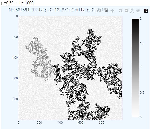
        global cc;    cc +=0.02;    B = np.where(R < cc, 1, 0);    B1=logical_not(B)*1;    lw, num = measurements.label(B);    w=np.max(lw);    area = measurements.sum(B, lw, index=arange(lw.max() + 1));    sB=B.sum();    w1=np.max(area);    ix=[i for i, x in enumerate(area) if x == w1];    a = np.array(ix);        C = np.where(lw ==a[0], 1, 0);        C1 = logical_not(C)*1;    D=B1+C1;        ama = logical_not(D)*1;        sama=ama.sum();        p=sB/(N*N);     im = ax1.imshow(D, cmap=cmap, interpolation='nearest'); 
        with out:
            ax2.plot(p,sama/sB,'ro-');        display(ax1.figure);        print("p= ",p, "c= ",sB,"LC= ",sama," Author: S.Boutiche");        clear_output(wait=True);
    
    ax2.set_xticks(np.arange(-0.0, 1, 0.1));ax2.set_yticks(np.arange(-0.0, 1, 0.1));ax2.set_xlim([0,1.0]);ax2.set_ylim([0,1.0]);ax2.grid();plt2.title('Percolation function');plt2.grid();ax2.set_xlabel('percolation probability (percolation threshold at pc=0.5927)');ax2.set_ylabel(r'$\theta$(p)');    
    button.on_click(click);
    click(None);


    3. Jupyter python repository

    In another github repository, is released the jupyter code that can be run on the Binder environment (mybinder.org). two apps are presented:
  • perco.ipynb (simulation of this web application)
  • square_perco.ipynb (simulation of N by N, N=variable, square site percolation application) To run it, just click the "launch binder" logo in the following "python-percolation" github repository